Creating Computer vision datasets
How to create a new novel datasets from a few set of images.

this project makes use of a residual network to classify different classes of fish based on images.
# install missing packages
!pip -q install torchsummary
import numpy as np
import pandas as pd
import seaborn as sns
import matplotlib.pyplot as plt
import matplotlib
import os
import torch
import torch.nn as nn
import torchvision.transforms as transforms
from torch.utils.data import DataLoader, Dataset, random_split
from torchvision.datasets import ImageFolder
from torchvision.utils import make_grid
from torchsummary import summary
from tqdm import tqdm
from sklearn.metrics import accuracy_score, confusion_matrix, classification_report
from pathlib import Path


# set background color to white
matplotlib.rcParams['figure.facecolor'] = '#ffffff'

# set default figure size
matplotlib.rcParams['figure.figsize'] = (15, 7)
DATA_DIR = r'../input/a-large-scale-fish-dataset/Fish_Dataset/Fish_Dataset'
exploring the images and their classes before modeling
# Get filepaths and labels
image_dir = Path(DATA_DIR)
filepaths = list(image_dir.glob(r'**/*.png'))
labels = list(map(lambda x: os.path.split(os.path.split(x)[0])[1], filepaths))

filepaths = pd.Series(filepaths, name='Filepath').astype(str)
labels = pd.Series(labels, name='Label')

# Concatenate filepaths and labels
image_df = pd.concat([filepaths, labels], axis=1)

# remove GT from some label names
image_df['Label'] = image_df['Label'].apply(lambda x: x.replace(" GT", ""))
image_df
| Filepath | Label | |
|---|---|---|
| 0 | ../input/a-large-scale-fish-dataset/Fish_Datas... | Hourse Mackerel |
| 1 | ../input/a-large-scale-fish-dataset/Fish_Datas... | Hourse Mackerel |
| 2 | ../input/a-large-scale-fish-dataset/Fish_Datas... | Hourse Mackerel |
| 3 | ../input/a-large-scale-fish-dataset/Fish_Datas... | Hourse Mackerel |
| 4 | ../input/a-large-scale-fish-dataset/Fish_Datas... | Hourse Mackerel |
| ... | ... | ... |
| 17995 | ../input/a-large-scale-fish-dataset/Fish_Datas... | Red Sea Bream |
| 17996 | ../input/a-large-scale-fish-dataset/Fish_Datas... | Red Sea Bream |
| 17997 | ../input/a-large-scale-fish-dataset/Fish_Datas... | Red Sea Bream |
| 17998 | ../input/a-large-scale-fish-dataset/Fish_Datas... | Red Sea Bream |
| 17999 | ../input/a-large-scale-fish-dataset/Fish_Datas... | Red Sea Bream |
18000 rows × 2 columns
# count plot for each class
sns.countplot(x='Label', data=image_df).set(title='Count of different image classes')
plt.show()
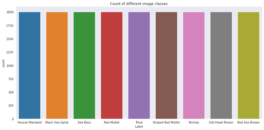
there are 2000 images of each class, which means our model won’t be biased towereds a particular class because it has a larger sample size
# the images are already augumented so no need to do any transforms
trans = transforms.Compose([transforms.Resize([128, 128]), # resize to a smaller size to avoid CUDA running out of memory
                            transforms.ToTensor()
                           ])

images = ImageFolder(root=DATA_DIR, transform=trans)
# split data to train, test
size = len(images)
test_size = int(0.2 * size)
train_size = int(size - test_size)
print(f"number of classes: {len(images.classes)}")
print(f"total number of images: {size}")
print(f"total number of train images: {train_size}")
print(f"total number of test images: {test_size}")
# random_split
train_set, test_set = random_split(images, (train_size, test_size))
number of classes: 9
total number of images: 18000
total number of train images: 14400
total number of test images: 3600
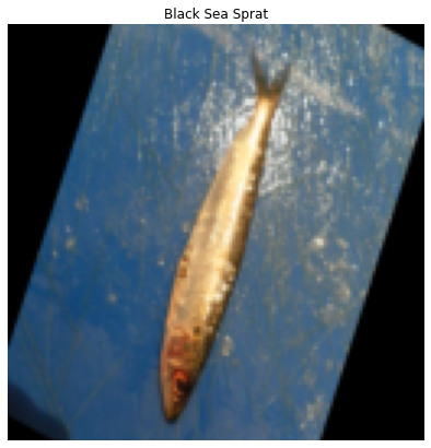
# show a single image
def show_image(img, label, dataset):
    plt.imshow(img.permute(1, 2, 0))
    plt.axis('off')
    plt.title(dataset.classes[label])
show_image(*train_set[7], train_set.dataset)
show_image(*train_set[101], train_set.dataset)
# create data loaders
batch_size = 64 # larger numbers lead to CUDA running out of memory
train_dl = DataLoader(train_set, batch_size=batch_size)
test_dl = DataLoader(test_set, batch_size=batch_size)
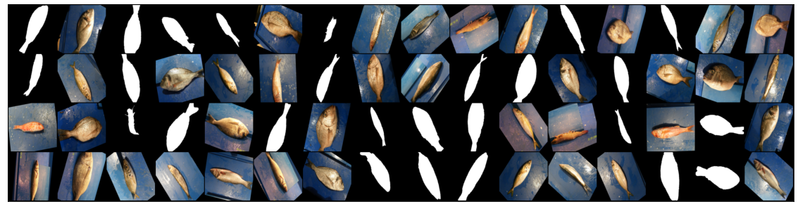
# visualize a batch of images
def show_batch(dl):
    for images, labels in dl:
        fig, ax = plt.subplots(figsize=(20, 8))
        ax.set_xticks([]); ax.set_yticks([])
        ax.imshow(make_grid(images, nrow=16).permute(1, 2, 0))
        break
show_batch(train_dl)
# convlutional block with batchnorm and max pooling
def conv_block(in_channels, out_channels, pool=False):
    layers = [nn.Conv2d(in_channels, out_channels, kernel_size=3, padding=1),
              nn.BatchNorm2d(out_channels),
              nn.ReLU(inplace=True)]
    if pool: layers.append(nn.MaxPool2d(2))
    return nn.Sequential(*layers)


# CNN with residual connections
class FishResNet(nn.Module):
    def __init__(self, in_channels, num_classes):
        super().__init__()

        self.conv1 = conv_block(in_channels, 64)
        self.conv2 = conv_block(64, 128, pool=True)
        self.res1 = nn.Sequential(conv_block(128, 128), conv_block(128, 128))

        self.conv3 = conv_block(128, 256, pool=True)
        self.conv4 = conv_block(256, 512, pool=True)
        self.res2 = nn.Sequential(conv_block(512, 512), conv_block(512, 512))

        self.classifier = nn.Sequential(nn.MaxPool2d(4),
                                        nn.Flatten(),
                                        nn.Dropout(0.2),
                                        nn.Linear(512 * 4 * 4, num_classes))

    def forward(self, xb):
        out = self.conv1(xb)
        out = self.conv2(out)
        out = self.res1(out) + out # add residual
        out = self.conv3(out)
        out = self.conv4(out)
        out = self.res2(out) + out # add residual
        out = self.classifier(out)
        return out
device = torch.device('cuda' if torch.cuda.is_available() else 'cpu') # choose device accordingly
model = FishResNet(3, 9).to(device) # 3 color channels and 9 output classes
criterion = nn.CrossEntropyLoss()
optim = torch.optim.Adam(model.parameters(), lr=1e-3)

# model summary (helps in understanding the output shapes)
summary(model, (3, 128, 128))
----------------------------------------------------------------
        Layer (type)               Output Shape         Param #
================================================================
            Conv2d-1         [-1, 64, 128, 128]           1,792
       BatchNorm2d-2         [-1, 64, 128, 128]             128
              ReLU-3         [-1, 64, 128, 128]               0
            Conv2d-4        [-1, 128, 128, 128]          73,856
       BatchNorm2d-5        [-1, 128, 128, 128]             256
              ReLU-6        [-1, 128, 128, 128]               0
         MaxPool2d-7          [-1, 128, 64, 64]               0
            Conv2d-8          [-1, 128, 64, 64]         147,584
       BatchNorm2d-9          [-1, 128, 64, 64]             256
             ReLU-10          [-1, 128, 64, 64]               0
           Conv2d-11          [-1, 128, 64, 64]         147,584
      BatchNorm2d-12          [-1, 128, 64, 64]             256
             ReLU-13          [-1, 128, 64, 64]               0
           Conv2d-14          [-1, 256, 64, 64]         295,168
      BatchNorm2d-15          [-1, 256, 64, 64]             512
             ReLU-16          [-1, 256, 64, 64]               0
        MaxPool2d-17          [-1, 256, 32, 32]               0
           Conv2d-18          [-1, 512, 32, 32]       1,180,160
      BatchNorm2d-19          [-1, 512, 32, 32]           1,024
             ReLU-20          [-1, 512, 32, 32]               0
        MaxPool2d-21          [-1, 512, 16, 16]               0
           Conv2d-22          [-1, 512, 16, 16]       2,359,808
      BatchNorm2d-23          [-1, 512, 16, 16]           1,024
             ReLU-24          [-1, 512, 16, 16]               0
           Conv2d-25          [-1, 512, 16, 16]       2,359,808
      BatchNorm2d-26          [-1, 512, 16, 16]           1,024
             ReLU-27          [-1, 512, 16, 16]               0
        MaxPool2d-28            [-1, 512, 4, 4]               0
          Flatten-29                 [-1, 8192]               0
          Dropout-30                 [-1, 8192]               0
           Linear-31                    [-1, 9]          73,737
================================================================
Total params: 6,643,977
Trainable params: 6,643,977
Non-trainable params: 0
----------------------------------------------------------------
Input size (MB): 0.19
Forward/backward pass size (MB): 145.19
Params size (MB): 25.34
Estimated Total Size (MB): 170.72
----------------------------------------------------------------
# multiclass accuracy
def multi_acc(y_pred, y_test):
    y_pred_softmax = torch.log_softmax(y_pred, dim = 1)
    _, y_pred_tags = torch.max(y_pred_softmax, dim = 1)
    correct_pred = (y_pred_tags == y_test).float()
    acc = correct_pred.sum() / len(correct_pred)
    acc = torch.round(acc * 100)
    return acc
# training loop
epochs = 10
losses = []
for epoch in range(epochs):
    # for custom progress bar
    with tqdm(train_dl, unit="batch") as tepoch:
        epoch_loss = 0
        for data, target in tepoch:
            tepoch.set_description(f"Epoch {epoch + 1}")
            data, target = data.to(device), target.to(device) # move input to GPU
            out = model(data)
            loss = criterion(out, target)
            acc = multi_acc(out, target)
            epoch_loss += loss.item()
            loss.backward()
            optim.step()
            optim.zero_grad()
            tepoch.set_postfix(loss = loss.item(), accuracy = acc.item()) # show loss and accuracy per batch of data
    losses.append(epoch_loss)
Epoch 1: 100%|██████████| 225/225 [04:55<00:00,  1.31s/batch, accuracy=45, loss=1.57]
Epoch 2: 100%|██████████| 225/225 [02:52<00:00,  1.30batch/s, accuracy=67, loss=0.914]
Epoch 3: 100%|██████████| 225/225 [02:51<00:00,  1.31batch/s, accuracy=75, loss=0.822]
Epoch 4: 100%|██████████| 225/225 [02:52<00:00,  1.31batch/s, accuracy=81, loss=0.414]
Epoch 5: 100%|██████████| 225/225 [02:54<00:00,  1.29batch/s, accuracy=84, loss=0.38]
Epoch 6: 100%|██████████| 225/225 [02:55<00:00,  1.29batch/s, accuracy=83, loss=0.37]
Epoch 7: 100%|██████████| 225/225 [02:56<00:00,  1.28batch/s, accuracy=88, loss=0.385]
Epoch 8: 100%|██████████| 225/225 [02:55<00:00,  1.28batch/s, accuracy=84, loss=0.325]
Epoch 9: 100%|██████████| 225/225 [02:56<00:00,  1.28batch/s, accuracy=89, loss=0.343]
Epoch 10: 100%|██████████| 225/225 [02:56<00:00,  1.28batch/s, accuracy=91, loss=0.186]
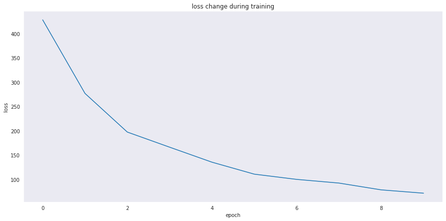
we can see that the batch loss is decreasing on each epoch meaning the model is learning effectively, the accuracy also keeps raising the longer we train, to make the loss easier to understand lets plot it
# plot losses
sns.set_style("dark")
sns.lineplot(data=losses).set(title="loss change during training", xlabel="epoch", ylabel="loss")
plt.show()
# predict on testing data samples (the accuracy here is batch accuracy)
y_pred_list = []
y_true_list = []
with torch.no_grad():
    with tqdm(test_dl, unit="batch") as tepoch:
        for inp, labels in tepoch:
            inp, labels = inp.to(device), labels.to(device)
            y_test_pred = model(inp)
            acc = multi_acc(y_test_pred, labels)
            _, y_pred_tag = torch.max(y_test_pred, dim = 1)
            tepoch.set_postfix(accuracy = acc.item())
            y_pred_list.append(y_pred_tag.cpu().numpy())
            y_true_list.append(labels.cpu().numpy())
100%|██████████| 57/57 [00:35<00:00, 1.60batch/s, accuracy=75]
# flatten prediction and true lists
flat_pred = []
flat_true = []
for i in range(len(y_pred_list)):
    for j in range(len(y_pred_list[i])):
        flat_pred.append(y_pred_list[i][j])
        flat_true.append(y_true_list[i][j])

print(f"number of testing samples results: {len(flat_pred)}")
number of testing samples results: 3600
# calculate total testing accuracy
print(f"Testing accuracy is: {accuracy_score(flat_true, flat_pred) * 100:.2f}%")
Testing accuracy is: 87.11%
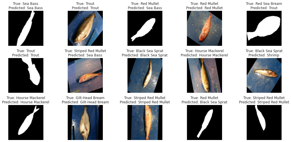
# Display 15 random picture of the dataset with their labels
inds = np.random.randint(len(test_set), size=15)
fig, axes = plt.subplots(nrows=3, ncols=5, figsize=(15, 7),
                        subplot_kw={'xticks': [], 'yticks': []})

for i, ax in zip(inds, axes.flat):
    img, label = test_set[i]
    ax.imshow(img.permute(1, 2, 0))
    ax.set_title(f"True: {test_set.dataset.classes[label]}\nPredicted: {test_set.dataset.classes[flat_pred[i]]}")
plt.tight_layout()
plt.show()
# classification report
print(classification_report(flat_true, flat_pred, target_names=images.classes))
                    precision    recall  f1-score   support

   Black Sea Sprat       0.88      0.85      0.87       428
   Gilt-Head Bream       0.88      0.84      0.86       412
   Hourse Mackerel       0.99      0.91      0.95       403
        Red Mullet       0.79      0.91      0.84       391
     Red Sea Bream       0.86      0.88      0.87       406
          Sea Bass       0.87      0.94      0.90       364
            Shrimp       0.81      1.00      0.90       420
Striped Red Mullet       0.97      0.55      0.70       392
             Trout       0.87      0.95      0.91       384

          accuracy                           0.87      3600
         macro avg       0.88      0.87      0.87      3600
      weighted avg       0.88      0.87      0.87      3600
# plot confusion matrix
idx2class = {v: k for k, v in images.class_to_idx.items()}
confusion_matrix_df = pd.DataFrame(confusion_matrix(flat_true, flat_pred)).rename(columns=idx2class, index=idx2class)
sns.heatmap(confusion_matrix_df, annot=True, fmt='').set(title="confusion matrix", xlabel="Predicted Label", ylabel="True Label")
plt.show()
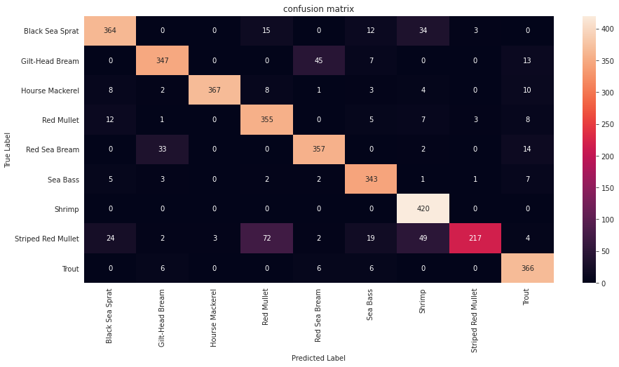
in this project we classified 9 different classes of fish at an decent accuracy of 87% with most of the classes having good percision and recall, however the model can be improved further by employing some techniques such as:
How to create a new novel datasets from a few set of images.
Data Science Project

Data Science Project

A Decentralized Application that simulates a bank using blockchain