Creating Computer vision datasets
How to create a new novel datasets from a few set of images.

import pandas as pd
import numpy as np
import seaborn as sns
import torch
import torch.nn as nn
import torch.nn.functional as F
from torch.utils.data import DataLoader
from torch.utils.data import TensorDataset
import matplotlib.pyplot as plt
from sklearn.model_selection import train_test_split
from sklearn.metrics import accuracy_score, confusion_matrix, classification_report
from sklearn.preprocessing import StandardScaler

# set default figure size
plt.rcParams['figure.figsize'] = (15, 7.0)
heart_data = '../input/heart-attack-analysis-prediction-dataset/heart.csv'

heart_df = pd.read_csv(heart_data)

heart_df.head()
| age | sex | cp | trtbps | chol | fbs | restecg | thalachh | exng | oldpeak | slp | caa | thall | output | |
|---|---|---|---|---|---|---|---|---|---|---|---|---|---|---|
| 0 | 63 | 1 | 3 | 145 | 233 | 1 | 0 | 150 | 0 | 2.3 | 0 | 0 | 1 | 1 |
| 1 | 37 | 1 | 2 | 130 | 250 | 0 | 1 | 187 | 0 | 3.5 | 0 | 0 | 2 | 1 |
| 2 | 41 | 0 | 1 | 130 | 204 | 0 | 0 | 172 | 0 | 1.4 | 2 | 0 | 2 | 1 |
| 3 | 56 | 1 | 1 | 120 | 236 | 0 | 1 | 178 | 0 | 0.8 | 2 | 0 | 2 | 1 |
| 4 | 57 | 0 | 0 | 120 | 354 | 0 | 1 | 163 | 1 | 0.6 | 2 | 0 | 2 | 1 |
# describe the data
heart_df.describe()
| age | sex | cp | trtbps | chol | fbs | restecg | thalachh | exng | oldpeak | slp | caa | thall | output | |
|---|---|---|---|---|---|---|---|---|---|---|---|---|---|---|
| count | 303.000000 | 303.000000 | 303.000000 | 303.000000 | 303.000000 | 303.000000 | 303.000000 | 303.000000 | 303.000000 | 303.000000 | 303.000000 | 303.000000 | 303.000000 | 303.000000 |
| mean | 54.366337 | 0.683168 | 0.966997 | 131.623762 | 246.264026 | 0.148515 | 0.528053 | 149.646865 | 0.326733 | 1.039604 | 1.399340 | 0.729373 | 2.313531 | 0.544554 |
| std | 9.082101 | 0.466011 | 1.032052 | 17.538143 | 51.830751 | 0.356198 | 0.525860 | 22.905161 | 0.469794 | 1.161075 | 0.616226 | 1.022606 | 0.612277 | 0.498835 |
| min | 29.000000 | 0.000000 | 0.000000 | 94.000000 | 126.000000 | 0.000000 | 0.000000 | 71.000000 | 0.000000 | 0.000000 | 0.000000 | 0.000000 | 0.000000 | 0.000000 |
| 25% | 47.500000 | 0.000000 | 0.000000 | 120.000000 | 211.000000 | 0.000000 | 0.000000 | 133.500000 | 0.000000 | 0.000000 | 1.000000 | 0.000000 | 2.000000 | 0.000000 |
| 50% | 55.000000 | 1.000000 | 1.000000 | 130.000000 | 240.000000 | 0.000000 | 1.000000 | 153.000000 | 0.000000 | 0.800000 | 1.000000 | 0.000000 | 2.000000 | 1.000000 |
| 75% | 61.000000 | 1.000000 | 2.000000 | 140.000000 | 274.500000 | 0.000000 | 1.000000 | 166.000000 | 1.000000 | 1.600000 | 2.000000 | 1.000000 | 3.000000 | 1.000000 |
| max | 77.000000 | 1.000000 | 3.000000 | 200.000000 | 564.000000 | 1.000000 | 2.000000 | 202.000000 | 1.000000 | 6.200000 | 2.000000 | 4.000000 | 3.000000 | 1.000000 |
# checking data types
heart_df.dtypes
age           int64
sex           int64
cp            int64
trtbps        int64
chol          int64
fbs           int64
restecg       int64
thalachh      int64
exng          int64
oldpeak     float64
slp           int64
caa           int64
thall         int64
output        int64
dtype: object
# drop duplicates if any
heart_df.drop_duplicates()

# check missing valus
heart_df.isna().sum()
age         0
sex         0
cp          0
trtbps      0
chol        0
fbs         0
restecg     0
thalachh    0
exng        0
oldpeak     0
slp         0
caa         0
thall       0
output      0
dtype: int64
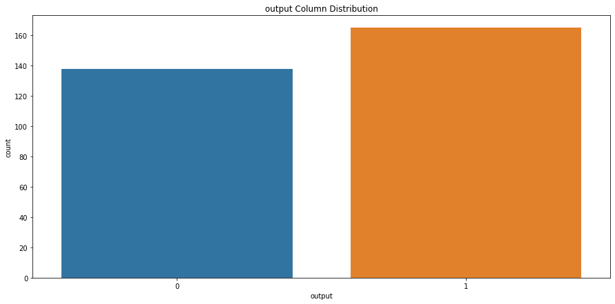
# check output column class distribution
sns.countplot(x='output', data=heart_df).set_title("output Column Distribution")
Text(0.5, 1.0, 'output Column Distribution')
# check sex column class distribution
sns.countplot(x='sex', data=heart_df).set_title("Sex Column Distribution")
Text(0.5, 1.0, 'Sex Column Distribution')

# box plot for output and cholestrol level
sns.boxplot(x="output",y="chol",data=heart_df)
<AxesSubplot:xlabel='output', ylabel='chol'>

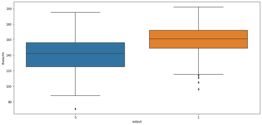
# box plot for output and cholestrol level
sns.boxplot(x="output",y="thalachh",data=heart_df)
<AxesSubplot:xlabel='output', ylabel='thalachh'>
# box plot for output and cholestrol level
sns.boxplot(x="output",y="oldpeak",data=heart_df)
<AxesSubplot:xlabel='output', ylabel='oldpeak'>

# box plot for output and cholestrol level
sns.boxplot(x="output",y="age",data=heart_df)
<AxesSubplot:xlabel='output', ylabel='age'>

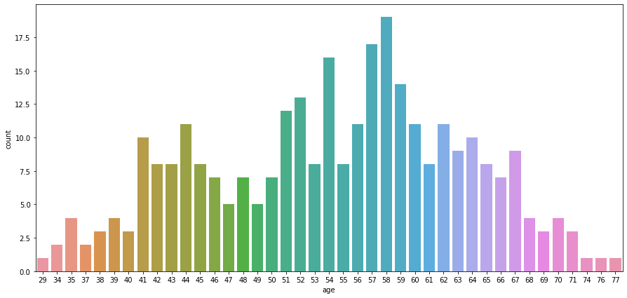
ax = sns.countplot(x='age', data=heart_df)
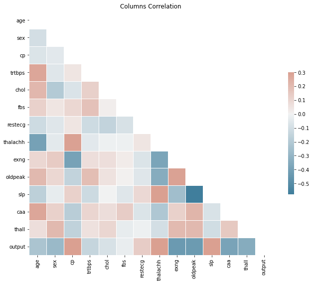
# check correlation
corr = heart_df.corr()

# Generate a mask for the upper triangle
mask = np.triu(np.ones_like(corr, dtype=bool))

# Set up the matplotlib figure
f, ax = plt.subplots(figsize=(11, 9))

# Generate a custom diverging colormap
cmap = sns.diverging_palette(230, 20, as_cmap=True)

# Draw the heatmap with the mask and correct aspect ratio
sns.heatmap(corr, mask=mask, cmap=cmap, vmax=.3, center=0,
            square=True, linewidths=.5, cbar_kws={"shrink": .5}).set_title("Columns Correlation")
Text(0.5, 1.0, 'Columns Correlation')
# split data for training
y = heart_df.output.to_numpy()
X = heart_df.drop('output', axis=1).to_numpy()

# scale X values
scaler = StandardScaler()
X = scaler.fit_transform(X)

# split data while keeping output class distribution consistent
X_train, X_test, y_train, y_test = train_test_split(X, y, test_size=0.2, stratify=y)
# convert data to pytorch tensors
def df_to_tensor(df):
    return torch.from_numpy(df).float()

X_traint = df_to_tensor(X_train)
y_traint = df_to_tensor(y_train)
X_testt = df_to_tensor(X_test)
y_testt = df_to_tensor(y_test)
# create pytorch dataset
train_ds = TensorDataset(X_traint, y_traint)
test_ds = TensorDataset(X_testt, y_testt)

# create data loaders
batch_size = 5
train_dl = DataLoader(train_ds, batch_size, shuffle=True)
test_dl = DataLoader(test_ds, batch_size, shuffle=False)
# model architecture
class BinaryNetwork(nn.Module):
    def __init__(self, input_size, output_size):
        super().__init__()
        self.l1 = nn.Linear(input_size, 64)
        self.l2 = nn.Linear(64, 32)
        self.l3 = nn.Linear(32, 16)
        self.out = nn.Linear(16, output_size)

    def forward(self, x):
        x = self.l1(x)
        x = F.relu(x)
        x = self.l2(x)
        x = F.relu(x)
        x = self.l3(x)
        x = F.relu(x)
        x = self.out(x)
        return torch.sigmoid(x) # scaling values between 0 and 1
input_size = 13 # number of features
output_size = 1
model = BinaryNetwork(input_size, output_size)
loss_fn = nn.BCELoss() # Binary Cross Entropy
optim = torch.optim.Adam(model.parameters(), lr=1e-3)
model
BinaryNetwork(
  (l1): Linear(in_features=13, out_features=64, bias=True)
  (l2): Linear(in_features=64, out_features=32, bias=True)
  (l3): Linear(in_features=32, out_features=16, bias=True)
  (out): Linear(in_features=16, out_features=1, bias=True)
)
epochs = 100
losses = []
for i in range(epochs):
    epoch_loss = 0
    for feat, target in train_dl:
        optim.zero_grad()
        out = model(feat)
        loss = loss_fn(out, target.unsqueeze(1))
        epoch_loss += loss.item()
        loss.backward()
        optim.step()
    losses.append(epoch_loss)
    # print loss every 10
    if i % 10 == 0:
        print(f"Epoch: {i}/{epochs}, Loss = {loss:.5f}")
Epoch: 0/100, Loss = 0.79641
Epoch: 10/100, Loss = 0.03637
Epoch: 20/100, Loss = 0.07704
Epoch: 30/100, Loss = 0.02023
Epoch: 40/100, Loss = 0.00084
Epoch: 50/100, Loss = 0.00000
Epoch: 60/100, Loss = 0.00001
Epoch: 70/100, Loss = 0.00000
Epoch: 80/100, Loss = 0.00018
Epoch: 90/100, Loss = 0.00029
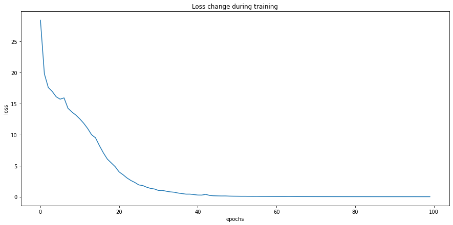
# plot losses
graph = sns.lineplot(x=[x for x in range(0, epochs)], y=losses)
graph.set(title="Loss change during training", xlabel='epochs', ylabel='loss')
plt.show()
# evaluate the model
y_pred_list = []
model.eval()
with torch.no_grad():
    for X, y in test_dl:
        y_test_pred = model(X)
        y_pred_tag = torch.round(y_test_pred)
        y_pred_list.append(y_pred_tag)

# convert predictions to a list of tensors with 1 dimention
y_pred_list = [a.squeeze() for a in y_pred_list]
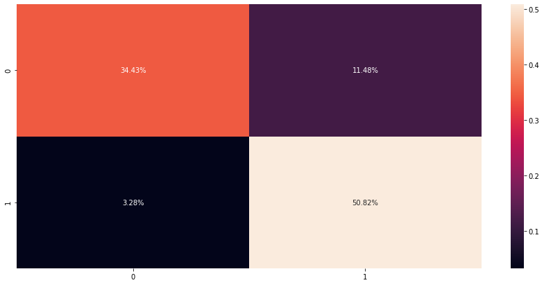
# check confusion matrix (hstack will merge all tensor lists into one list)
cfm = confusion_matrix(y_test, torch.hstack(y_pred_list))
sns.heatmap(cfm / np.sum(cfm), annot=True, fmt='.2%')
<AxesSubplot:>
# print metrics
print(classification_report(y_test, torch.hstack(y_pred_list)))
              precision    recall  f1-score   support

           0       0.91      0.75      0.82        28
           1       0.82      0.94      0.87        33

    accuracy                           0.85        61
   macro avg       0.86      0.84      0.85        61
weighted avg       0.86      0.85      0.85        61
How to create a new novel datasets from a few set of images.
Data Science Project

Data Science Project

A Decentralized Application that simulates a bank using blockchain