Creating Computer vision datasets
How to create a new novel datasets from a few set of images.

lazy predict is a library that trains a large number of models on a given dataset to determine which one will work best for it
the goal is to predict a price range for a smartphone based on its specifications.
the specifcations include a total of 20 columns ranging from 3g availability to touch screen and amount of ram so a very extensive feature set.
import numpy as np
import pandas as pd
import matplotlib.pyplot as plt
from matplotlib.pyplot import figure
import seaborn as sns
train = pd.read_csv("../input/mobile-price-classification/train.csv")
test = pd.read_csv("../input/mobile-price-classification/test.csv")
after loading in the data, lets take a look at it
train.head()
| battery_power | blue | clock_speed | dual_sim | fc | four_g | int_memory | m_dep | mobile_wt | n_cores | ... | px_height | px_width | ram | sc_h | sc_w | talk_time | three_g | touch_screen | wifi | price_range | |
|---|---|---|---|---|---|---|---|---|---|---|---|---|---|---|---|---|---|---|---|---|---|
| 0 | 842 | 0 | 2.2 | 0 | 1 | 0 | 7 | 0.6 | 188 | 2 | ... | 20 | 756 | 2549 | 9 | 7 | 19 | 0 | 0 | 1 | 1 |
| 1 | 1021 | 1 | 0.5 | 1 | 0 | 1 | 53 | 0.7 | 136 | 3 | ... | 905 | 1988 | 2631 | 17 | 3 | 7 | 1 | 1 | 0 | 2 |
| 2 | 563 | 1 | 0.5 | 1 | 2 | 1 | 41 | 0.9 | 145 | 5 | ... | 1263 | 1716 | 2603 | 11 | 2 | 9 | 1 | 1 | 0 | 2 |
| 3 | 615 | 1 | 2.5 | 0 | 0 | 0 | 10 | 0.8 | 131 | 6 | ... | 1216 | 1786 | 2769 | 16 | 8 | 11 | 1 | 0 | 0 | 2 |
| 4 | 1821 | 1 | 1.2 | 0 | 13 | 1 | 44 | 0.6 | 141 | 2 | ... | 1208 | 1212 | 1411 | 8 | 2 | 15 | 1 | 1 | 0 | 1 |
5 rows × 21 columns
test.head()
| id | battery_power | blue | clock_speed | dual_sim | fc | four_g | int_memory | m_dep | mobile_wt | ... | pc | px_height | px_width | ram | sc_h | sc_w | talk_time | three_g | touch_screen | wifi | |
|---|---|---|---|---|---|---|---|---|---|---|---|---|---|---|---|---|---|---|---|---|---|
| 0 | 1 | 1043 | 1 | 1.8 | 1 | 14 | 0 | 5 | 0.1 | 193 | ... | 16 | 226 | 1412 | 3476 | 12 | 7 | 2 | 0 | 1 | 0 |
| 1 | 2 | 841 | 1 | 0.5 | 1 | 4 | 1 | 61 | 0.8 | 191 | ... | 12 | 746 | 857 | 3895 | 6 | 0 | 7 | 1 | 0 | 0 |
| 2 | 3 | 1807 | 1 | 2.8 | 0 | 1 | 0 | 27 | 0.9 | 186 | ... | 4 | 1270 | 1366 | 2396 | 17 | 10 | 10 | 0 | 1 | 1 |
| 3 | 4 | 1546 | 0 | 0.5 | 1 | 18 | 1 | 25 | 0.5 | 96 | ... | 20 | 295 | 1752 | 3893 | 10 | 0 | 7 | 1 | 1 | 0 |
| 4 | 5 | 1434 | 0 | 1.4 | 0 | 11 | 1 | 49 | 0.5 | 108 | ... | 18 | 749 | 810 | 1773 | 15 | 8 | 7 | 1 | 0 | 1 |
5 rows × 21 columns
# check data types
train.info()
<class 'pandas.core.frame.DataFrame'>
RangeIndex: 2000 entries, 0 to 1999
Data columns (total 21 columns):
 #   Column         Non-Null Count  Dtype
---  ------         --------------  -----
 0   battery_power  2000 non-null   int64
 1   blue           2000 non-null   int64
 2   clock_speed    2000 non-null   float64
 3   dual_sim       2000 non-null   int64
 4   fc             2000 non-null   int64
 5   four_g         2000 non-null   int64
 6   int_memory     2000 non-null   int64
 7   m_dep          2000 non-null   float64
 8   mobile_wt      2000 non-null   int64
 9   n_cores        2000 non-null   int64
 10  pc             2000 non-null   int64
 11  px_height      2000 non-null   int64
 12  px_width       2000 non-null   int64
 13  ram            2000 non-null   int64
 14  sc_h           2000 non-null   int64
 15  sc_w           2000 non-null   int64
 16  talk_time      2000 non-null   int64
 17  three_g        2000 non-null   int64
 18  touch_screen   2000 non-null   int64
 19  wifi           2000 non-null   int64
 20  price_range    2000 non-null   int64
dtypes: float64(2), int64(19)
memory usage: 328.2 KB
# check if there are any null columns
train.isna().sum()
battery_power    0
blue             0
clock_speed      0
dual_sim         0
fc               0
four_g           0
int_memory       0
m_dep            0
mobile_wt        0
n_cores          0
pc               0
px_height        0
px_width         0
ram              0
sc_h             0
sc_w             0
talk_time        0
three_g          0
touch_screen     0
wifi             0
price_range      0
dtype: int64
# describe the data
train.describe()
| battery_power | blue | clock_speed | dual_sim | fc | four_g | int_memory | m_dep | mobile_wt | n_cores | ... | px_height | px_width | ram | sc_h | sc_w | talk_time | three_g | touch_screen | wifi | price_range | |
|---|---|---|---|---|---|---|---|---|---|---|---|---|---|---|---|---|---|---|---|---|---|
| count | 2000.000000 | 2000.0000 | 2000.000000 | 2000.000000 | 2000.000000 | 2000.000000 | 2000.000000 | 2000.000000 | 2000.000000 | 2000.000000 | ... | 2000.000000 | 2000.000000 | 2000.000000 | 2000.000000 | 2000.000000 | 2000.000000 | 2000.000000 | 2000.000000 | 2000.000000 | 2000.000000 |
| mean | 1238.518500 | 0.4950 | 1.522250 | 0.509500 | 4.309500 | 0.521500 | 32.046500 | 0.501750 | 140.249000 | 4.520500 | ... | 645.108000 | 1251.515500 | 2124.213000 | 12.306500 | 5.767000 | 11.011000 | 0.761500 | 0.503000 | 0.507000 | 1.500000 |
| std | 439.418206 | 0.5001 | 0.816004 | 0.500035 | 4.341444 | 0.499662 | 18.145715 | 0.288416 | 35.399655 | 2.287837 | ... | 443.780811 | 432.199447 | 1084.732044 | 4.213245 | 4.356398 | 5.463955 | 0.426273 | 0.500116 | 0.500076 | 1.118314 |
| min | 501.000000 | 0.0000 | 0.500000 | 0.000000 | 0.000000 | 0.000000 | 2.000000 | 0.100000 | 80.000000 | 1.000000 | ... | 0.000000 | 500.000000 | 256.000000 | 5.000000 | 0.000000 | 2.000000 | 0.000000 | 0.000000 | 0.000000 | 0.000000 |
| 25% | 851.750000 | 0.0000 | 0.700000 | 0.000000 | 1.000000 | 0.000000 | 16.000000 | 0.200000 | 109.000000 | 3.000000 | ... | 282.750000 | 874.750000 | 1207.500000 | 9.000000 | 2.000000 | 6.000000 | 1.000000 | 0.000000 | 0.000000 | 0.750000 |
| 50% | 1226.000000 | 0.0000 | 1.500000 | 1.000000 | 3.000000 | 1.000000 | 32.000000 | 0.500000 | 141.000000 | 4.000000 | ... | 564.000000 | 1247.000000 | 2146.500000 | 12.000000 | 5.000000 | 11.000000 | 1.000000 | 1.000000 | 1.000000 | 1.500000 |
| 75% | 1615.250000 | 1.0000 | 2.200000 | 1.000000 | 7.000000 | 1.000000 | 48.000000 | 0.800000 | 170.000000 | 7.000000 | ... | 947.250000 | 1633.000000 | 3064.500000 | 16.000000 | 9.000000 | 16.000000 | 1.000000 | 1.000000 | 1.000000 | 2.250000 |
| max | 1998.000000 | 1.0000 | 3.000000 | 1.000000 | 19.000000 | 1.000000 | 64.000000 | 1.000000 | 200.000000 | 8.000000 | ... | 1960.000000 | 1998.000000 | 3998.000000 | 19.000000 | 18.000000 | 20.000000 | 1.000000 | 1.000000 | 1.000000 | 3.000000 |
8 rows × 21 columns
# number of samples for each price range
fig, ax = plt.subplots(figsize = (10, 4))
sns.countplot(x ='price_range', data=train)
plt.xlabel("Class Label")
plt.ylabel("Number of Samples")
plt.show()
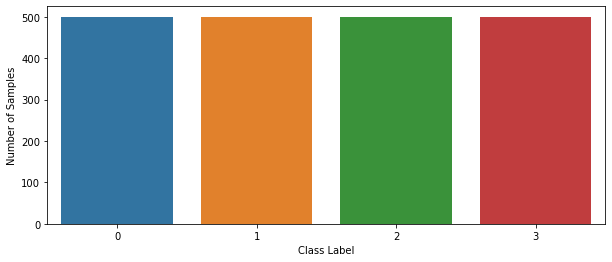
perfectly balanced, as all things should be.
# find correlation
corr_mat = train.corr()

# each columns correlation with the price
corr_mat['price_range']
battery_power    0.200723
blue             0.020573
clock_speed     -0.006606
dual_sim         0.017444
fc               0.021998
four_g           0.014772
int_memory       0.044435
m_dep            0.000853
mobile_wt       -0.030302
n_cores          0.004399
pc               0.033599
px_height        0.148858
px_width         0.165818
ram              0.917046
sc_h             0.022986
sc_w             0.038711
talk_time        0.021859
three_g          0.023611
touch_screen    -0.030411
wifi             0.018785
price_range      1.000000
Name: price_range, dtype: float64
# convert all to positive and sort by value
abs(corr_mat).sort_values(by=['price_range'])['price_range']
m_dep            0.000853
n_cores          0.004399
clock_speed      0.006606
four_g           0.014772
dual_sim         0.017444
wifi             0.018785
blue             0.020573
talk_time        0.021859
fc               0.021998
sc_h             0.022986
three_g          0.023611
mobile_wt        0.030302
touch_screen     0.030411
pc               0.033599
sc_w             0.038711
int_memory       0.044435
px_height        0.148858
px_width         0.165818
battery_power    0.200723
ram              0.917046
price_range      1.000000
Name: price_range, dtype: float64
we can make a few observations from above
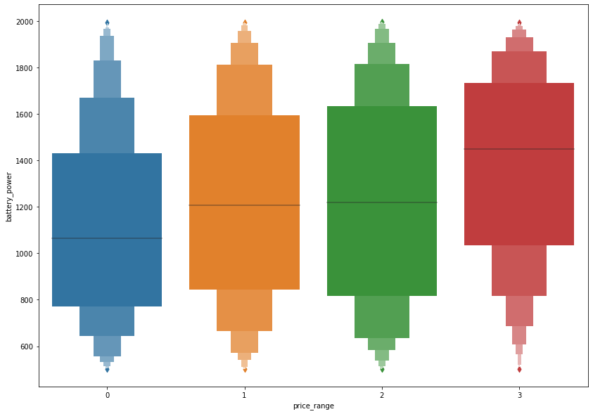
# battery correlation plot
fig, ax = plt.subplots(figsize=(14,10))
sns.boxenplot(x="price_range",y="battery_power", data=train,ax = ax)
<matplotlib.axes._subplots.AxesSubplot at 0x7fa979ba8dd0>
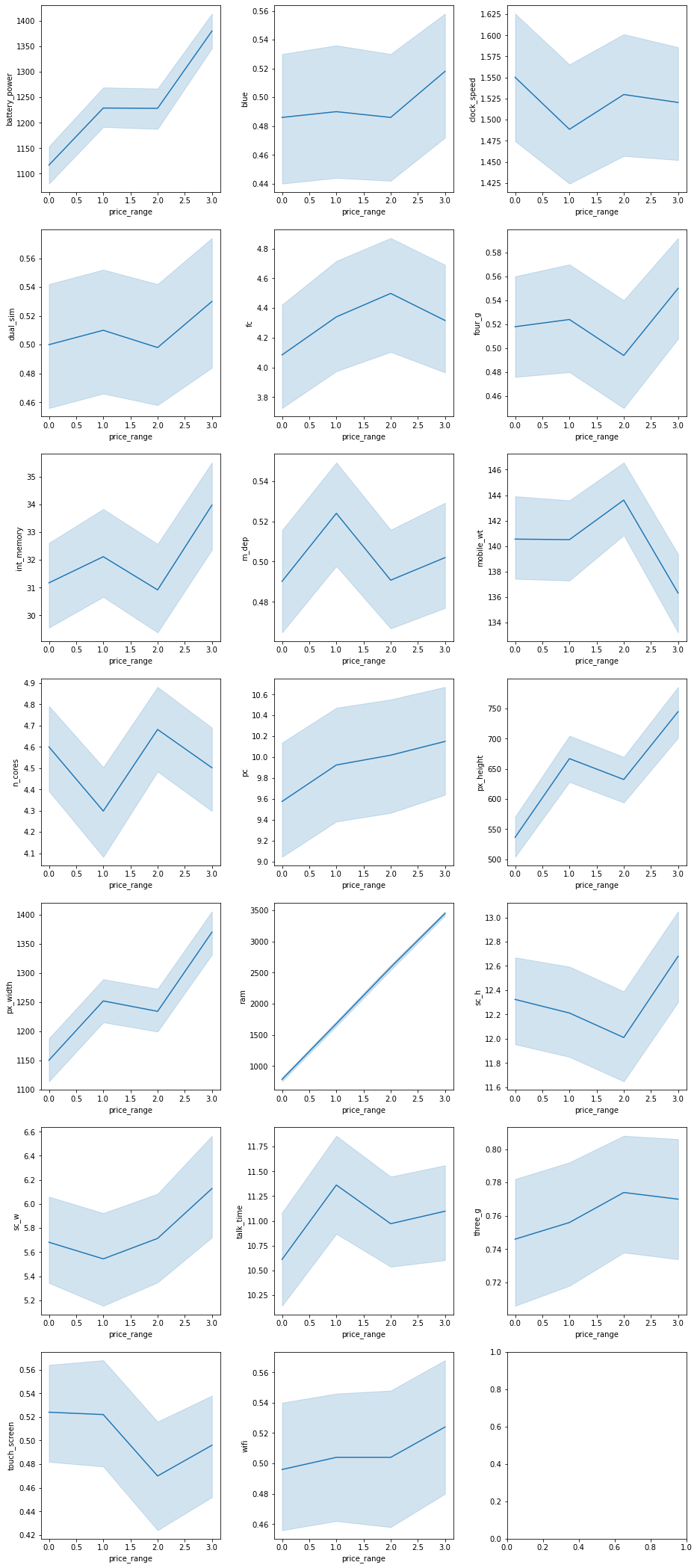
# individual correlation graphs

# get all columns and remove price_range
cols = list(train.columns.values)
cols.remove('price_range')

# plot figure
fig, ax = plt.subplots(7, 3, figsize=(15, 30))
plt.subplots_adjust(left=0.1, bottom=0.05, top=1.0, wspace=0.3, hspace=0.2)
for i, col in zip(range(len(cols)), cols):
    ax = plt.subplot(7,3,i+1)
    sns.lineplot(ax=ax,x='price_range', y=col, data=train)
# plot full heatmap
figure(figsize=(20, 14))
sns.heatmap(corr_mat, annot = True, fmt='.1g', cmap= 'coolwarm')
<matplotlib.axes._subplots.AxesSubplot at 0x7fa9771fd850>
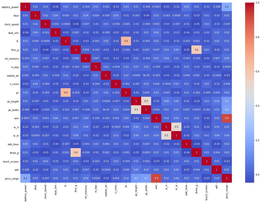
knowing which model to build for a dataset is not an easy task, specially when the columns that have a high correlation with the target variable are less than half the total columns, its also a task that is time consuming in making and tuning these models that is why we will use the LazyPredict library to show us the results of various models without any tuneing and we will implement the top 3 models.
# extract target column
target = train['price_range']

# drop target column from dataset
train.drop('price_range', axis=1, inplace=True)
from sklearn.model_selection import train_test_split

# install and import lazypredict
!pip install lazypredict
from lazypredict.Supervised import LazyClassifier

# split training dataset to training and testing
X_train, X_test, y_train, y_test = train_test_split(train, target,test_size=.3,random_state =123)

# make Lazyclassifier model(s)
lazy_clf = LazyClassifier(verbose=0, ignore_warnings=True, custom_metric=None)

# fit model(s)
models, predictions = lazy_clf.fit(X_train, X_test, y_train, y_test)
Requirement already satisfied: lazypredict in /opt/conda/lib/python3.7/site-packages (0.2.7)
Requirement already satisfied: Click>=7.0 in /opt/conda/lib/python3.7/site-packages (from lazypredict) (7.1.1)
[33mWARNING: You are using pip version 20.3.1; however, version 20.3.3 is available.
You should consider upgrading via the '/opt/conda/bin/python3.7 -m pip install --upgrade pip' command.[0m
100%|██████████| 30/30 [00:04<00:00, 6.21it/s]
models
| Accuracy | Balanced Accuracy | ROC AUC | F1 Score | Time Taken | |
|---|---|---|---|---|---|
| Model | |||||
| LogisticRegression | 0.94 | 0.95 | None | 0.94 | 0.06 |
| LinearDiscriminantAnalysis | 0.93 | 0.93 | None | 0.93 | 0.07 |
| QuadraticDiscriminantAnalysis | 0.92 | 0.92 | None | 0.92 | 0.02 |
| LGBMClassifier | 0.91 | 0.91 | None | 0.91 | 0.48 |
| XGBClassifier | 0.91 | 0.91 | None | 0.90 | 0.41 |
| RandomForestClassifier | 0.87 | 0.87 | None | 0.87 | 0.50 |
| SVC | 0.86 | 0.87 | None | 0.86 | 0.17 |
| NuSVC | 0.86 | 0.87 | None | 0.86 | 0.22 |
| BaggingClassifier | 0.86 | 0.87 | None | 0.86 | 0.13 |
| ExtraTreesClassifier | 0.84 | 0.85 | None | 0.84 | 0.37 |
| DecisionTreeClassifier | 0.84 | 0.84 | None | 0.84 | 0.03 |
| LinearSVC | 0.82 | 0.83 | None | 0.82 | 0.32 |
| CalibratedClassifierCV | 0.81 | 0.82 | None | 0.80 | 1.06 |
| GaussianNB | 0.78 | 0.79 | None | 0.78 | 0.02 |
| PassiveAggressiveClassifier | 0.74 | 0.75 | None | 0.74 | 0.03 |
| SGDClassifier | 0.73 | 0.74 | None | 0.72 | 0.05 |
| Perceptron | 0.73 | 0.74 | None | 0.73 | 0.03 |
| NearestCentroid | 0.70 | 0.70 | None | 0.70 | 0.02 |
| AdaBoostClassifier | 0.63 | 0.62 | None | 0.61 | 0.22 |
| RidgeClassifier | 0.56 | 0.58 | None | 0.47 | 0.04 |
| RidgeClassifierCV | 0.56 | 0.58 | None | 0.47 | 0.02 |
| BernoulliNB | 0.53 | 0.54 | None | 0.52 | 0.03 |
| KNeighborsClassifier | 0.52 | 0.52 | None | 0.52 | 0.08 |
| ExtraTreeClassifier | 0.51 | 0.51 | None | 0.51 | 0.02 |
| LabelSpreading | 0.45 | 0.45 | None | 0.45 | 0.20 |
| LabelPropagation | 0.45 | 0.45 | None | 0.45 | 0.15 |
| DummyClassifier | 0.26 | 0.26 | None | 0.26 | 0.02 |
| CheckingClassifier | 0.25 | 0.25 | None | 0.10 | 0.02 |
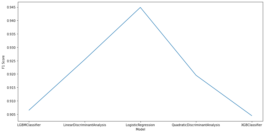
# plot the first 5 models F1 score
top = models[:5]
figure(figsize=(14, 7))
sns.lineplot(x=top.index, y="F1 Score", data=top)
<matplotlib.axes._subplots.AxesSubplot at 0x7fa946d44bd0>
we are not really intrested in the predictions dataframe here because we already know those values and they’re part of the training dataset
from above we can see that the best algorithm for this type of task is logistic regression followed by Discriminant Analysis models and followed closely by GB models.
the reason behing skipping on the Quadratic Discriminant Analysis model is because its of the same family as Linear Discriminant Analysis and produces similar results, we also want to implement a diverse range of models
from sklearn.linear_model import LogisticRegression
# Logistic regression
log_clf = LogisticRegression(random_state=0).fit(train, target)
# drop the id column from test to match the size of train
test.drop('id', axis=1, inplace=True)
# get predictions on test dataset and convert it to a dataframe
log_preds = pd.DataFrame(log_clf.predict(test), columns = ['log_price_range'])

log_preds.head()
| log_price_range | |
|---|---|
| 0 | 2 |
| 1 | 3 |
| 2 | 2 |
| 3 | 3 |
| 4 | 2 |
from sklearn.discriminant_analysis import LinearDiscriminantAnalysis
# Linear Discriminant Analysis
lda_clf = LinearDiscriminantAnalysis().fit(train, target)
# get predictions on test dataset and convert it to a dataframe
lda_preds = pd.DataFrame(lda_clf.predict(test), columns = ['lda_price_range'])

lda_preds.head()
| lda_price_range | |
|---|---|
| 0 | 3 |
| 1 | 3 |
| 2 | 2 |
| 3 | 3 |
| 4 | 1 |
from lightgbm import LGBMClassifier
# lightgbm model
lgbm_clf = LGBMClassifier(objective='multiclass', random_state=5).fit(train, target)
# get predictions on test dataset and convert it to a dataframe
lgbm_preds = pd.DataFrame(lgbm_clf.predict(test), columns = ['lgbm_price_range'])

lgbm_preds.head()
| lgbm_price_range | |
|---|---|
| 0 | 3 |
| 1 | 3 |
| 2 | 3 |
| 3 | 3 |
| 4 | 1 |
# create dataframe with 3 columns and index from any of the predicted dataframes
results = pd.DataFrame(index=log_preds.index, columns=['log', 'lda', 'lgbm'])

# add in data from the 3 predicted dfs
results['log'] = log_preds
results['lda'] = lda_preds
results['lgbm'] = lgbm_preds

# show grouped df
results
| log | lda | lgbm | |
|---|---|---|---|
| 0 | 2 | 3 | 3 |
| 1 | 3 | 3 | 3 |
| 2 | 2 | 2 | 3 |
| 3 | 3 | 3 | 3 |
| 4 | 2 | 1 | 1 |
| ... | ... | ... | ... |
| 995 | 1 | 2 | 2 |
| 996 | 1 | 1 | 1 |
| 997 | 2 | 0 | 0 |
| 998 | 1 | 2 | 2 |
| 999 | 3 | 2 | 2 |
1000 rows × 3 columns
# find columns where all 3 models agree on the result
equal_rows = 0
for row in results.itertuples(index=False):
    if(row.log == row.lda == row.lgbm):
        equal_rows += 1

equal_rows
628
from all the 1000 rows the 3 models agree on 62% which means any of these 3 algorithms should be n overall good choice for predicting the price range of a smartphone based on its specifications
How to create a new novel datasets from a few set of images.
Data Science Project

Data Science Project

A Decentralized Application that simulates a bank using blockchain